44 show data labels excel

How to create Custom Data Labels in Excel Charts - Efficiency 365 Create the chart as usual. Add default data labels. Click on each unwanted label (using slow double click) and delete it. Select each item where you want the custom label one at a time. Press F2 to move focus to the Formula editing box. Type the equal to sign. Now click on the cell which contains the appropriate label. Add a DATA LABEL to ONE POINT on a chart in Excel Steps shown in the video above: Click on the chart line to add the data point to. All the data points will be highlighted. Click again on the single point that you want to add a data label to. Right-click and select ' Add data label ' This is the key step! Right-click again on the data point itself (not the label) and select ' Format data label '.

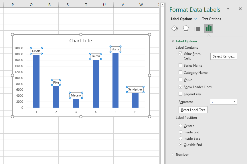
How to add data labels from different column in an Excel chart? Right click the data series, and select Format Data Labels from the context menu. 3. In the Format Data Labels pane, under Label Options tab, check the Value From Cells option, select the specified column in the popping out dialog, and click the OK button. Now the cell values are added before original data labels in bulk. 4.

Show data labels excel

How to show percentage in pie chart in Excel? - ExtendOffice Show percentage in pie chart in Excel. Please do as follows to create a pie chart and show percentage in the pie slices. 1. Select the data you will create a pie chart based on, click Insert > Insert Pie or Doughnut Chart > Pie. See screenshot: 2. Then a pie chart is created. Right click the pie chart and select Add Data Labels from the context ... How to Change Excel Chart Data Labels to Custom Values? May 05, 2010 · Now, click on any data label. This will select “all” data labels. Now click once again. At this point excel will select only one data label. Go to Formula bar, press = and point to the cell where the data label for that chart data point is defined. Repeat the process for all other data labels, one after another. See the screencast. How to Show Percentages in Stacked Column Chart in Excel? 17/12/2021 · Follow the below steps to show percentages in stacked column chart In Excel: Step 1: Open excel and create a data table as below. Step 2: Select the entire data table. Step 3: To create a column chart in excel for your data table. Go to “Insert” >> “Column or Bar Chart” >> Select Stacked Column Chart . Step 4: Add Data labels to the ...

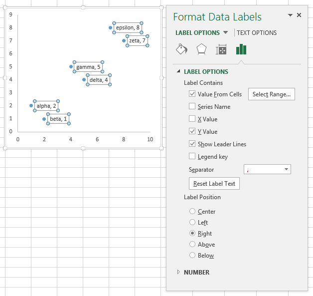
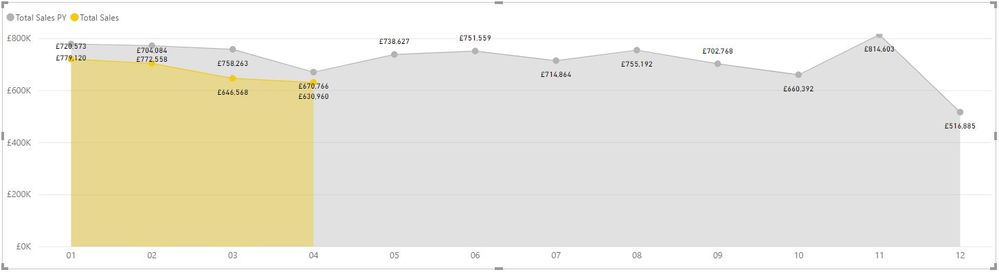
Show data labels excel. Find, label and highlight a certain data point in Excel scatter graph Select the Data Labels box and choose where to position the label. By default, Excel shows one numeric value for the label, y value in our case. To display both x and y values, right-click the label, click Format Data Labels…, select the X Value and Y value boxes, and set the Separator of your choosing: Label the data point by name Display Data Label for first & last data points [SOLVED] Re: Display Data Label for first & last data points. My suggestion using a pivot table. However, data is in another layout in the "Data" sheet. When you add more data, simply refresh the pivot table (Data Sheet - Refresh). From the PivotTable Filter, select the Year you want to show on the graphs. Attached Files. How to Add Data Labels to an Excel 2010 Chart - dummies On the Chart Tools Layout tab, click Data Labels→More Data Label Options. The Format Data Labels dialog box appears. You can use the options on the Label Options, Number, Fill, Border Color, Border Styles, Shadow, Glow and Soft Edges, 3-D Format, and Alignment tabs to customize the appearance and position of the data labels. Displaying Large Numbers in K (thousands) or M (millions) in Excel How To Display Numbers in Millions in Excel Right-Click any number you want to convert. Go to Format Cells. In the pop-up window, move to Custom formatting. If you want to show the numbers in Millions, simply change the format from General to 0,,"M" . The figures will now be 23M.

Create a map: easily map multiple locations from excel data Add pin labels to your map by selecting an option from a drop down menu. Map pin labels allow for locations to be quickly identified. They can be used to show fixed numbers, zip codes, prices, or any other data you want to see right on the map. Pin labels can be hidden by changing the Pin Label Zoom option. Create Dynamic Chart Data Labels with Slicers - Excel Campus Feb 10, 2016 · Step 3: Use the TEXT Function to Format the Labels. Typically a chart will display data labels based on the underlying source data for the chart. In Excel 2013 a new feature called “Value from Cells” was introduced. This feature allows us to specify the a range that we want to use for the labels. Where are data labels in Excel? - whathowinfo.com Add data labels to a chart Click the data series or chart. In the upper right corner, next to the chart, click Add Chart Element > Data Labels. To change the location, click the arrow, and choose an option. If you want to show your data label inside a text bubble shape, click Data Callout. Moreover, how do you move data labels in Excel? Change the format of data labels in a chart To get there, after adding your data labels, select the data label to format, and then click Chart Elements > Data Labels > More Options. To go to the appropriate area, click one of the four icons ( Fill & Line , Effects , Size & Properties ( Layout & Properties in Outlook or Word), or Label Options ) shown here.

How to show data label in "percentage" instead of - Microsoft Community Select Format Data Labels Select Number in the left column Select Percentage in the popup options In the Format code field set the number of decimal places required and click Add. (Or if the table data in in percentage format then you can select Link to source.) Click OK Regards, OssieMac Report abuse 8 people found this reply helpful · How to Add Total Data Labels to the Excel Stacked Bar Chart Apr 03, 2013 · Step 4: Right click your new line chart and select “Add Data Labels” Step 5: Right click your new data labels and format them so that their label position is “Above”; also make the labels bold and increase the font size. Step 6: Right click the line, select “Format Data Series”; in the Line Color menu, select “No line” to display top 5 data labels on graph [SOLVED] Re: to display top 5 data labels on graph. Also, I noticed your sum column ("total") is returning errors. I don't see why you would want to do this, and in fact I'm not even sure why excel wanted to do this to begin with. if you run C3+D3 when those cells are empty, excel should return 0. So I got rid of the error, and that way, you can use the ... Custom Chart Data Labels In Excel With Formulas - How To Excel At Excel Follow the steps below to create the custom data labels. Select the chart label you want to change. In the formula-bar hit = (equals), select the cell reference containing your chart label's data. In this case, the first label is in cell E2. Finally, repeat for all your chart laebls.

Custom data labels in a chart

Excel charts: how to move data labels to legend @Matt_Fischer-Daly . You can't do that, but you can show a data table below the chart instead of data labels: Click anywhere on the chart. On the Design tab of the ribbon (under Chart Tools), in the Chart Layouts group, click Add Chart Element > Data Table > With Legend Keys (or No Legend Keys if you prefer)

This is how you can add data labels in Power BI [EASY STEPS]

Format Data Labels in Excel- Instructions - TeachUcomp, Inc. To format data labels in Excel, choose the set of data labels to format. To do this, click the "Format" tab within the "Chart Tools" contextual tab in the Ribbon. Then select the data labels to format from the "Chart Elements" drop-down in the "Current Selection" button group. Then click the "Format Selection" button that ...

Chart axes, legend, data labels, trendline in Excel - Tech Funda

Data labels on small states using Maps - Microsoft Community Data labels on small states using Maps. Hello, I need some assistance using the Filled Maps chart type in Excel (note: this is NOT Power Maps). I have some data (see attachment below) that I've plotted on a map of the USA. Because the data only applied to 7 states I changed the "map area" (under Format Data Series-->Series Options) to show ...

Add or remove data labels in a chart

How To Create Labels In Excel - cgc-finances.info Click inside the chart area to display the chart tools. Create labels without having to copy your data. Make Row Labels In Excel 2007 Freeze For Easier Reading from Enter the randbetween excel function. How to use create cards. In the first cell of the text column, enter... Read More "How To Create Labels In Excel" »

Apply Custom Data Labels to Charted Points - Peltier Tech

How to Show Percentage in Pie Chart in Excel? - GeeksforGeeks 29/06/2021 · It can be observed that the pie chart contains the value in the labels but our aim is to show the data labels in terms of percentage. Show percentage in a pie chart: The steps are as follows : Select the pie chart. Right-click on it. A pop-down menu will appear. Click on the Format Data Labels option. The Format Data Labels dialog box will appear.

Presenting Data with Charts

How to hide zero data labels in chart in Excel? - ExtendOffice If you want to hide zero data labels in chart, please do as follow: 1. Right click at one of the data labels, and select Format Data Labels from the context menu. See screenshot: 2. In the Format Data Labels dialog, Click Number in left pane, then select Custom from the Category list box, and type #"" into the Format Code text box, and click Add button to add it to Type list box.

How to Add Two Data Labels in Excel Chart (with Easy Steps ...

DataLabels.ShowValue property (Excel) | Microsoft Docs Syntax expression. ShowValue expression A variable that represents a DataLabels object. Remarks The specified chart must first be active before you can access the data labels programmatically, or a run-time error will occur. Example This example enables the value to be shown for the data labels of the first series, on the first chart.

Adapting charts – empower® Support

How to Use Cell Values for Excel Chart Labels - How-To Geek Mar 12, 2020 · Make your chart labels in Microsoft Excel dynamic by linking them to cell values. When the data changes, the chart labels automatically update. In this article, we explore how to make both your chart title and the chart data labels dynamic. We have the sample data below with product sales and the difference in last month’s sales.

Move data labels

how to add data labels into Excel graphs - storytelling with data You can download the corresponding Excel file to follow along with these steps: Right-click on a point and choose Add Data Label. You can choose any point to add a label—I'm strategically choosing the endpoint because that's where a label would best align with my design. Excel defaults to labeling the numeric value, as shown below.

excel - How to show series-Legend label name in data labels ...

Excel tutorial: How to use data labels Generally, the easiest way to show data labels to use the chart elements menu. When you check the box, you'll see data labels appear in the chart. If you have more than one data series, you can select a series first, then turn on data labels for that series only. You can even select a single bar, and show just one data label.

How to Add Two Data Labels in Excel Chart (with Easy Steps ...

How to use data labels in a chart - YouTube Excel charts have a flexible system to display values called "data labels". Data labels are a classic example a "simple" Excel feature with a huge range of o...

Change the format of data labels in a chart

Chart.ApplyDataLabels method (Excel) | Microsoft Docs The type of data label to apply. True to show the legend key next to the point. The default value is False. True if the object automatically generates appropriate text based on content. For the Chart and Series objects, True if the series has leader lines. Pass a Boolean value to enable or disable the series name for the data label.

Change the format of data labels in a chart

Show or hide a chart legend or data table - support.microsoft.com Add or remove a secondary axis in a chart in Excel Article; Add a trend or moving average line to a chart Article; ... in the Labels group, click Data Table. Do one of the following: To display a data table, click Show Data Table or Show Data Table with Legend Keys.

Apply Custom Data Labels to Charted Points - Peltier Tech

Excel, giving data labels to only the top/bottom X% values 1) Create a data set next to your original series column with only the values you want labels for (again, this can be formula driven to only select the top / bottom n values). See column D below. 2) Add this data series to the chart and show the data labels. 3) Set the line color to No Line, so that it does not appear! 4) Volia! See Below! Share

microsoft excel - Adding data label only to the last value ...

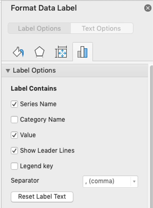
Add or remove data labels in a chart - support.microsoft.com Right-click the data series or data label to display more data for, and then click Format Data Labels. Click Label Options and under Label Contains, select the Values From Cells checkbox. When the Data Label Range dialog box appears, go back to the spreadsheet and select the range for which you want the cell values to display as data labels.

microsoft excel - Adding data label only to the last value ...

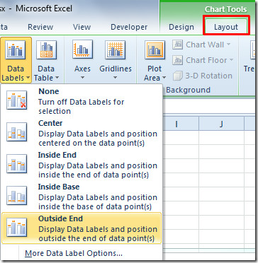
Adding Data Labels to Your Chart (Microsoft Excel) - ExcelTips (ribbon) Make sure the Design tab of the ribbon is displayed. (This will appear when the chart is selected.) Click the Add Chart Element drop-down list. Select the Data Labels tool. Excel displays a number of options that control where your data labels are positioned. Select the position that best fits where you want your labels to appear.

How To Show Or Hide Data Labels On MS Excel? | My Windows Hub

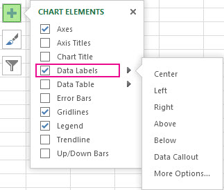
How to Add Data Labels in Excel - Excelchat | Excelchat In Excel 2013 and the later versions we need to do the followings; Click anywhere in the chart area to display the Chart Elements button Figure 5. Chart Elements Button Click the Chart Elements button > Select the Data Labels, then click the Arrow to choose the data labels position. Figure 6. How to Add Data Labels in Excel 2013 Figure 7.

Format Data Labels in Excel- Instructions - TeachUcomp, Inc.

How to add data labels in excel to graph or chart (Step-by-Step) Add data labels to a chart. 1. Select a data series or a graph. After picking the series, click the data point you want to label. 2. Click Add Chart Element Chart Elements button > Data Labels in the upper right corner, close to the chart. 3. Click the arrow and select an option to modify the location. 4.

Add or remove data labels in a chart

How to Make a Pie Chart in Excel & Add Rich Data Labels to ... 08/09/2022 · One can add rich data labels to data points or one point solely of a chart. Adding a rich data label linked to a certain cell is useful when you want to highlight a certain point on a chart or convey more information about this particular point. ... Excel Pie Chart Labels on Slices: Add, Show & Modify Factors; How to Change Pie Chart Colors in ...

Change the format of data labels in a chart

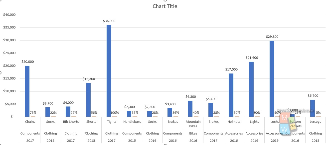
How to Show Percentages in Stacked Column Chart in Excel? 17/12/2021 · Follow the below steps to show percentages in stacked column chart In Excel: Step 1: Open excel and create a data table as below. Step 2: Select the entire data table. Step 3: To create a column chart in excel for your data table. Go to “Insert” >> “Column or Bar Chart” >> Select Stacked Column Chart . Step 4: Add Data labels to the ...

Change the format of data labels in a chart

How to Change Excel Chart Data Labels to Custom Values? May 05, 2010 · Now, click on any data label. This will select “all” data labels. Now click once again. At this point excel will select only one data label. Go to Formula bar, press = and point to the cell where the data label for that chart data point is defined. Repeat the process for all other data labels, one after another. See the screencast.